You have a variant effect prediction task in a diagnostic lab. Or perhaps you need to call somatic mutations in a tumour, spot a gene fusion in RNA, confirm a splice variant in a child with a suspected inherited disorder, or identify a pathogen in cerebrospinal fluid. Every month brings another genomic foundation model with an impressive benchmark table. Which one—if any—should you actually use?
First, a plain definition. Unlike task-specific tools built for a single job (such as SpliceAI for splice sites or Mutect2 for somatic calling), a foundation model is a neural network pretrained on massive collections of unlabelled DNA or RNA sequences. By learning to fill in masked bases or predict the next base across billions or trillions of nucleotides, it learns general sequence patterns without clinical labels. Once pretrained, the same model can score whether a mutation makes a DNA sequence look less plausible, produce numerical sequence summaries (embeddings) for a lightweight classifier, or be fine-tuned on your own labelled dataset.
What the model papers rarely tell you is how these models compare against the tools a diagnostic lab already runs. Reviewing the published evidence across eight routine diagnostic sequencing tasks alongside post-calling variant effect evaluations reveals a clear pattern:
- Across the eight diagnostic tasks, five had no published study comparing a foundation model against the established workflow baseline, two liquid-biopsy tasks had only preliminary evidence, and in the one independent threshold-transfer test on patient RNA-confirmed splice variants, SpliceAI achieved the highest sensitivity (88.2% at 99.1% specificity) across the five models scored at the intended variant coordinates.12
- Where foundation models do earn a look is post-calling variant effect scoring and custom DNA sequence classification—provided you test against current baselines on held-out splits, pick the right model size, pooling strategy, and prediction route, and account for single-GPU memory limits and cross-hardware numerical reproducibility.
This review walks through the task-first decision tree and the 2026 DNA models (Tables 1–2), why pretraining scale does not pick your model (Table 3), what independent research and clinical workflow benchmarks show (Table 4), hardware and memory requirements across models (Table 5), when to use zero-shot scoring versus frozen embeddings or fine-tuning (Table 6), and the key limitations for regulated clinical pipelines. All evidence was checked through 19 October 2026 (including the 24 GB L4 follow-up completed on 16 October).
The Decision Tree: What Are You Actually Trying to Do?
Start with your biological task, not with a model architecture. Calling a variant from raw sequencing reads, scoring whether an already-called variant disrupts gene function, and training a custom classifier on DNA sequences are three different jobs. Figure 1 maps the practical starting path for each one, and Table 1 (charted in Figure 2) summarises what my companion evidence reviews found across eight clinical diagnostic workflows plus post-calling variant scoring.

Figure 1. Decision tree for choosing between an established diagnostic pipeline, current variant effect predictors, and a DNA foundation model. Diagram by the author, synthesised from the companion evidence reviews linked below.
| Area | Task | Baseline named in the review | Foundation-model evidence in these reviews |
|---|---|---|---|
| Oncology | Tumour somatic SNVs and indels | Mutect2 | No comparison with the named baseline found |
| Oncology | Tumour RNA fusions | STAR-Fusion, Arriba | No comparison with the named baseline found |
| Oncology | ctDNA fragmentomics | ichorCNA tumour fraction | Fragmentia-AI, developers' test only |
| Oncology | ctDNA methylation | Elastic net (detection); constrained least-squares deconvolution such as MethAtlas (tissue of origin) | CpGPT, small internal tests with feature selection using the full cohort |
| Inherited disorders | Splice variants confirmed in patient RNA | Motif scoring such as MaxEntScan, then FRASER on RNA-seq; SpliceAI and Pangolin are the strongest predictors | Independent threshold-transfer test: SpliceAI had the highest sensitivity (88.2% at 99.1% specificity) |
| Oncology and inherited | Copy-number variants (CNVs) | ExomeDepth, CNVnator (calling); AnnotSV, ClassifyCNV (classification) | No comparison with the named baseline found |
| Infectious disease | DNA pathogen identification | Kraken2; minimap2 with MEGAN-LR | No comparison with the named baseline found |
| Infectious disease | RNA pathogen detection | Kraken2, Centrifuge | No machine-learning comparison with the named baseline found |
| Oncology and inherited | Variant effect scoring, after calling | CADD, AlphaMissense, GPN-MSA | Evo 2 embeddings competitive on ClinVar |
Table 1. Summary of established workflow baselines and foundation-model evidence across eight diagnostic sequencing tasks and post-calling variant effect scoring. Primary baseline and benchmark citations for each row are given in the task-by-task section below.
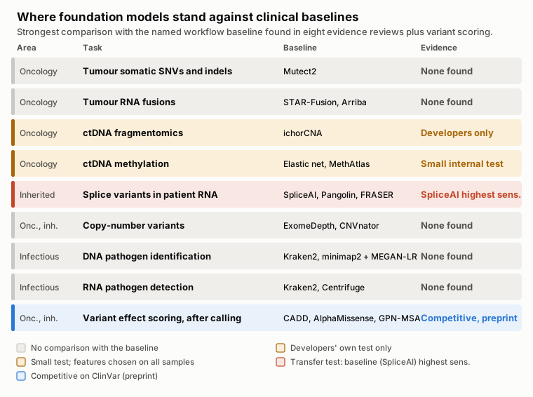
Figure 2. Table 1 as an evidence map: the strongest comparison between a foundation model and each task's named workflow baseline. Diagram by the author from the companion evidence reviews.
Table 1 records direct comparisons against established clinical workflow baselines, not every research paper that applies a model to sequences from the same domain. Where you do want to evaluate a DNA foundation model—either to score called variants or to build a sequence classifier—the 2026 landscape comes down to seven main model families (Table 2, Figure 3). They span five orders of magnitude in size, from under half a million to 40 billion parameters, and take sequence windows from a few kilobases (kb) to a full megabase (1 Mb).
| Model | Sizes | Longest input | Candidate use | Get it |
|---|---|---|---|---|
| DNABERT-2 | 117M | A few kb in practice | Short-sequence classification on modest GPUs | GitHub, Hugging Face |
| Nucleotide Transformer v2 | 50M to 500M | 12 kb | Short-sequence classification, cross-species work | GitHub |
| NTv3 | 8M to 650M | 1 Mb | Long inputs on one GPU | GitHub, Hugging Face |
| HyenaDNA | 0.44M to 6.6M | 1M bases | Very long inputs at low cost | GitHub, Hugging Face |
| Caduceus | About 0.5M to 7.7M | 131 kb | Human genome classification | GitHub |
| Evo 2 | 7B, 20B, 40B | 1 Mb | Variant effect scoring, generation | GitHub |
| AlphaGenome | n/a | 1 Mb | Predicting functional readouts of a variant | API, weights |
Table 2. Parameter counts, maximum input lengths, candidate diagnostic or research uses, and download links for major DNA sequence models in 2026. Primary model citations are given in the model-by-model summary immediately below.
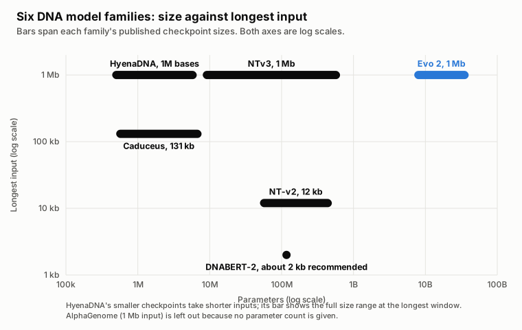
Figure 3. Parameter range against longest input for the model families in Table 2, on log scales. Plotted by the author from the sources in Table 2.
Which DNA Model Fits Your Task?
DNABERT-2 is the compact, fast starting point for short DNA sequences. In its authors' benchmark, it "achieves comparable performance to the state-of-the-art model with 21x fewer parameters and approximately 92x less GPU time in pre-training", where the comparator is the 2.5-billion-parameter Nucleotide Transformer.3 At 117M parameters, it replaces fixed -mer tokens with byte-pair encoding (BPE) that groups frequent multi-base runs into single tokens (Figure 4)—cutting token length roughly fivefold and enabling "efficient fine-tuning on most consumer GPUs".3 While the architecture has no hard length cap, Peng Wei, Chong Wu, and colleagues recommend keeping inputs to about 2 kb.4
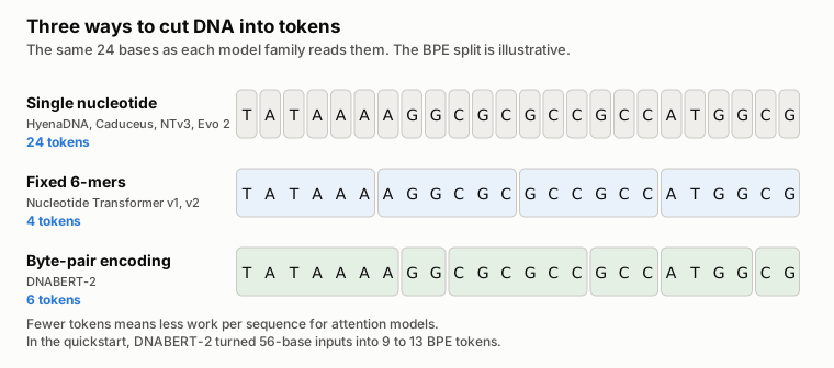
Figure 4. How single-nucleotide, fixed 6-mer and byte-pair encoding (BPE) tokenizers divide the same sequence. BPE boundaries are learned from data, so the split shown is illustrative. Diagram by the author.
Nucleotide Transformer (NT) spans three generations. The first generation scaled up to 2.5B parameters across 3,202 human genomes and 850 genomes from other species.5 Crucially, bigger was not better: in the authors' own benchmark, the second-generation 250M-parameter NT-v2 "attained the best performance on our benchmark (average MCC of 0.769) while being ten-times smaller than the 2.5B-parameter model" (where Matthews correlation coefficient, MCC, measures class agreement from to ).5 NT-v2 covers 50M to 500M parameters with a 12 kb window. The third generation, NTv3 (December 2025, 8M to 650M parameters), is designed to run full 1 Mb windows on a single A100 or H100 GPU.6
HyenaDNA was built for extreme sequence length. It handles "context lengths of up to 1 million tokens at the single nucleotide-level", "an up to 500x increase over previous dense attention-based models".7 At a sequence length of 1M tokens, it trains up to 160 times faster than a Transformer comparator.7 Not 1.6 times. One hundred and sixty (note that this is training speed in the authors' setup, not an inference ratio). The checkpoints are tiny, from 0.44M to 6.6M parameters.
A caveat on HyenaDNA. Long context does not guarantee higher accuracy on short-range biology. In independent evaluations, attention models beat HyenaDNA on short-range tasks, and HyenaDNA gained an edge only when tasks required long context.8 On BreCol, a 16S microbiome cancer-detection benchmark, HyenaDNA also trailed classical machine-learning methods on held-out data.9 When you do need long windows, pick the checkpoint carefully: the authors found (Appendix A.1) that a pretrained window 2 to 4 times longer than your downstream input works best.7
Caduceus builds DNA's reverse-complement symmetry directly into a state-space architecture that reads both strands while scaling linearly with sequence length (0.5M to 7.7M parameters, up to 131 kb).1011 In Feng and colleagues' independent benchmark, Caduceus-Ph was the strongest model overall across human genome classification tasks.4
Evo and Evo 2 are large generative models built on the StripedHyena architecture (which I examine in detail below). While the original 7B Evo was pretrained only on prokaryotic and phage sequences (131 kb window),12 Evo 2 trained on more than 8.8 trillion nucleotides across all domains of life in 7B, 20B, and 40B sizes with windows up to 1 Mb.1314 (A 1B checkpoint with an 8 kb window also exists,15 but the Evo 2 paper advises that it "should be avoided owing to overall weaker performance".13)
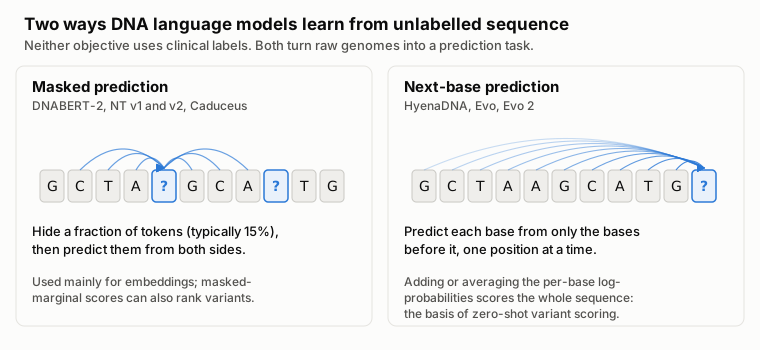
Figure 5. The two self-supervised pretraining objectives behind the language models in Table 2. Next-base models score a whole sequence directly, which is what zero-shot variant scoring uses. Diagram by the author.
AlphaGenome is a supervised sequence-to-function model rather than a self-supervised DNA language model (Figure 6): it predicts thousands of experimental tracks—gene expression, splicing, chromatin state, and 3D contacts—across a 1 Mb window, and its distilled model scores a variant in under a second on an H100 GPU.16 For ClinVar-style variant prioritisation where you want a single summary number rather than thousands of functional tracks, AlphaGenome Atlas precomputes the AlphaGenome Variant Impact (AVI) score across all possible human single-nucleotide variants.17 However, its free API and weights are restricted to non-commercial research (with commercial access via Google Cloud), and its terms state that predictions must not be used for clinical decision-making.1819
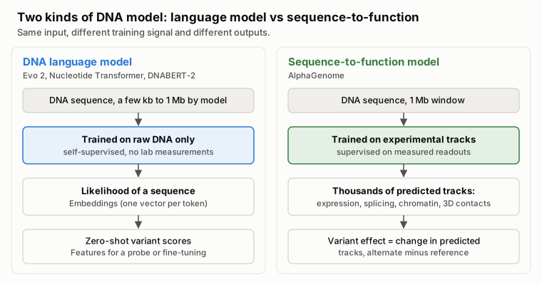
Figure 6. How a self-supervised DNA language model and a supervised sequence-to-function model differ in training signal and output. Diagram by the author.16
Other models you will see. GENA-LM (GitHub) accepts windows of about 4.5 kb or 36 kb.20 Genos (1.2B and 10B, up to 1 Mb) appears in the independent splicing test below;21 BGI subsequently released an updated checkpoint, Genos-10B-v2 (Hugging Face, 18 December 2025), trained with additional non-human primate and mammalian genomes and reporting improved RNA splicing prediction.22 GenomeOcean (100M to 4B) contributes H100 embedding memory figures in Table 5.23 All of these models have open weights or API access, but licences vary by checkpoint—check them before touching clinical workflows.
The Efficiency Revolution: Why Pretraining Scale Doesn't Pick Your Model
Pretraining a flagship genomic foundation model from scratch used to require a supercomputer cluster for a month. While a diagnostic lab will almost never pretrain from scratch, comparing the original pretraining runs (Table 3) reveals something vital for model selection: spending 100 times more compute during pretraining does not buy 100 times better downstream accuracy.
| Model | What the authors report | GPU-hours | At 13 October 2026 prices |
|---|---|---|---|
| Nucleotide Transformer 2.5B | 128 A100s for 28 days | 86,016 | about $154,000 |
| NTv3 650M | Pretraining and later stages on H100s | 8,920 | about $35,600 |
| HyenaDNA, 1M context | Up to 8 A100s for 4 weeks | up to 5,376 | up to about $9,600 |
| DNABERT-2 | 8 RTX 2080 Ti for about 14 days | 2,688 | about $1,300 |
| HyenaDNA, small | One A100 for 80 minutes | 1.3 | about $2 |
Table 3. Estimated cloud compute cost to pretrain five DNA foundation models from scratch, multiplying author-reported GPU-hours by 13 October 2026 Runpod secure-cloud on-demand prices (A100 80 GB $1.79/h, H100 $3.99/h; DNABERT-2's RTX 2080 Ti is priced at its faster RTX 3090 successor at $0.50/h; small HyenaDNA's A100 40 GB is priced at the 80 GB rate).24 My calculation, not what the authors paid; storage, networking, failed runs, and staff time are excluded. Sources: Nucleotide Transformer Methods;5 NTv3 Table 5;6 HyenaDNA Section 5, Appendix A.1 and Table A.2;7 DNABERT-2 Appendix A.3.3 (HyenaDNA Table A.2 lists a higher 215,000 GPU-hours for NT 2.5B; this table uses the Nucleotide Transformer paper's hardware figures.)
Look at the gap in Table 3 and Figure 7: pretraining DNABERT-2 took 32 times fewer raw GPU-hours than Nucleotide Transformer 2.5B (about $1,300 vs. $154,000 at current cloud rates), yet performed comparably on the DNABERT-2 benchmark.3 Within the Nucleotide Transformer family itself, the 250M NT-v2 beat the 2.5B model at one-tenth the parameter count.5 Smarter tokenization and updated training recipes matter far more than raw parameter count—and smaller models are much cheaper for your lab to run and adapt.
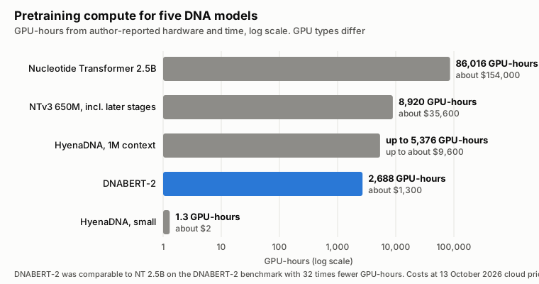
Figure 7. Pretraining GPU-hours from Table 3, derived from author-reported hardware and time, on a log scale, with my cloud cost estimates. DNABERT-2 used 32 times fewer GPU-hours than Nucleotide Transformer 2.5B and performed comparably on the DNABERT-2 benchmark.3
Benchmarks That Actually Matter: Research vs. Clinical Reality
Every model paper highlights benchmarks where its own architecture excels. Before trusting a headline score, examine two independent research benchmarks—Feng and colleagues4 and GenBench8—while keeping their scope in mind: both evaluate curated research sequence-classification datasets rather than clinical diagnostic endpoints, Feng and colleagues test frozen embeddings only (without fine-tuning or task-specific baselines), and model developers (including AlphaGenome's lead author) dispute how such multi-task suites construct and aggregate tasks into overall rankings. Where these suites are genuinely useful is in isolating design choices across shared splits—such as token pooling on frozen embeddings (confirmed by Feng and colleagues co-author Chong Wu) and how core layer families scale with input length—before you compare models against actual clinical diagnostic workflows.
The Pooling Strategy Secret
When a DNA foundation model reads a sequence of tokens, it outputs separate numerical vectors. To feed that sequence into a classifier, you must collapse those token vectors into a single vector per sequence (pooling). Most tutorials default to taking the single summary (CLS) token vector or the element-wise maximum (max pooling).
In their 2025 Nature Communications benchmark comparing DNABERT-2, NT-v2, HyenaDNA, Caduceus, and GROVER with frozen embeddings, Peng Wei and Chong Wu's groups at MD Anderson found a simple, consistent rule: "Mean token embedding consistently and significantly improves sequence classification performance, outperforming other pooling strategies."4 Averaging the vectors across all tokens (mean pooling, Figure 8) significantly beat summary-token and max pooling in 35 to 42 of 52 binary classification datasets, depending on the model.4 Start with mean pooling—averaging the hidden states across the token dimension—and verify alternatives on your validation split if you fine-tune.
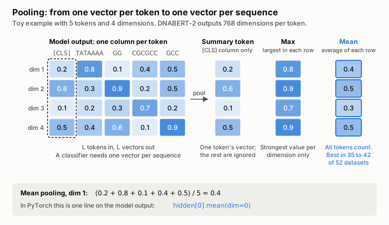
Figure 8. Three ways to pool per-token vectors into one sequence vector, shown on toy numbers. With frozen embeddings, Feng and colleagues found mean pooling significantly better than the other two in 35 to 42 of 52 binary classification datasets, depending on the model.4 Diagram by the author.
Attention vs. Convolution vs. State-Space Trade-offs
GenBench evaluates ten genomic models across 43 datasets, grouping them by how their core layers scale with sequence length (Figure 9):8
- Dense self-attention (
DNABERT-2,Nucleotide Transformer): compares every token against every other token, so pairwise attention computation grows quadratically as . Doubling the token count quadruples the pairwise attention calculation. - Long convolutions (
HyenaDNA): replace dense attention with implicit long convolutions evaluated via fast Fourier transforms in time.7 - State-space models (
Caduceus): scan along the sequence in linear time.108
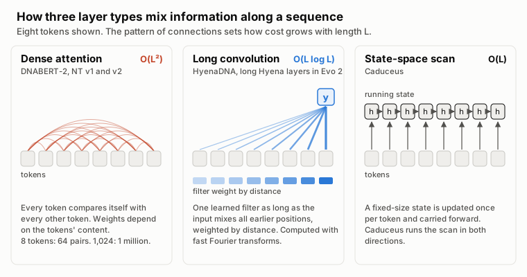
Figure 9. How dense attention, long convolution and state-space layers connect positions in a sequence, simplified. Figure 10 shows how the resulting work grows with input length. Diagram by the author from the HyenaDNA, Caduceus and GenBench papers.7108
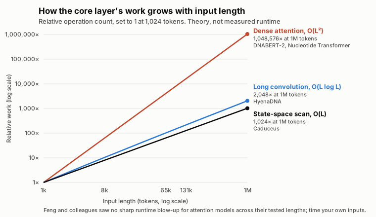
Figure 10. Theoretical growth in the core layer's work as input length increases, set to 1 at 1,024 tokens. These are operation counts from the complexity classes above, not measured runtimes; constant factors and GPU kernels decide real speed. Diagram by the author.
Two practical lessons emerge from the benchmarks. First, on short-range sequence tasks, dense-attention models consistently outperform convolution-based models in GenBench, whereas HyenaDNA catches up and leads on tasks that require long-range context (such as species classification at 450 kb to 1 Mb, where HyenaDNA reached 99.5% accuracy and standard Transformers could not be trained past 32 kb on the authors' hardware).78 Second, do not assume a fixed sequence length where attention suddenly hits a wall: when Feng and colleagues measured single-sequence inference (batch size 1) on an A100 GPU, none of the attention models showed a sharp quadratic runtime blow-up across their tested window lengths.4 Always time your actual input lengths on your own GPU.
Task-Specific Performance: Coding (1.5%), Noncoding (98.5%), and Eight Diagnostic Workflows
As GenBench highlights, protein-coding exons make up only about 1.5% of the human genome, while the remaining 98.5% is noncoding sequence (Figure 11) containing promoters, splice regions, enhancers, and structural elements.8 Models and baselines behave very differently across those regions—and even more differently when you move from curated research benchmarks to clinical diagnostic pipelines.
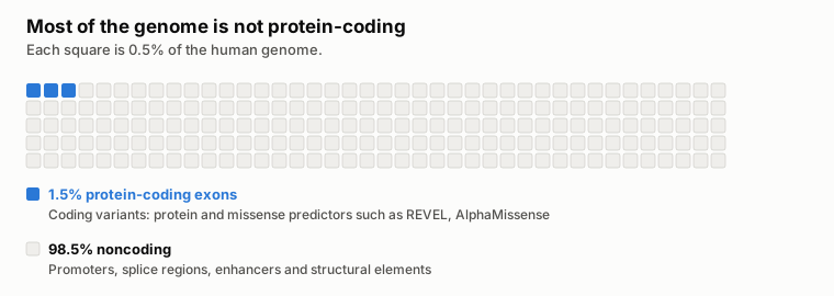
Figure 11. The human genome by function, using GenBench's 1.5% coding figure.8 Diagram by the author.
Here is what my eight companion clinical workflow reviews found when checking whether any genomic foundation model has beaten the established diagnostic tool:
- Tumour somatic SNVs and indels (Oncology): No foundation model was compared against the workflow baseline, Mutect2.25 Among task-specific deep-learning callers, DeepSomatic26 matched Mutect2 and beat Strelka227 in the only independent tumour-normal benchmark that included it,28 and NeuSomatic beat MuTect2 on SNV F1 score in 3 of 8 whole-genome pairs tested by Wang and colleagues.29 Keep Mutect2 (or hardware-accelerated Illumina DRAGEN3031) and evaluate deep-learning callers against it locally. Full review.
- Tumour RNA fusions (Oncology): No foundation-model or deep-learning caller was compared against STAR-Fusion32 or Arriba33 on the clinical workflow endpoint, including in Tamura and colleagues' 12-caller clinical RNA-seq benchmark.34 Full review.
- Detecting circulating tumour DNA (ctDNA) from fragmentomics (Oncology): Fragmentia-AI (a fragment model built on DNABERT-2) reported an AUROC of 0.956 versus at most 0.935 for DELFI fragment features35 in its developers' study,36 but has not been compared against ichorCNA,37 the standard tumour-fraction baseline. Promising, not yet proven. Full review.
- Detecting ctDNA and tissue of origin from DNA methylation (Oncology): Neither elastic-net detection nor constrained least-squares tissue-of-origin deconvolution (such as MethAtlas38) has been surpassed in an unconfounded foundation-model test. Xu and Feng fine-tuned CpGPT39 (a methylation foundation model they did not develop) and reported a mean test AUROC of 0.990 against 0.942 for elastic net and 0.957 for an SVM across three ~30-sample test splits.40 However, their Methods state that cancer-versus-control labels from all 300 samples were used to select the candidate CpG sites before splitting the cohort into training and test sets—a data-leakage limitation the authors acknowledge,40 which prevents knowing how much of CpGPT's lead would hold if feature selection were confined strictly to each training split. Full review.
- Detecting and classifying copy-number variants (Oncology and Inherited): No foundation model was evaluated against established CNV callers (ExomeDepth,41 CNVnator42) or clinical pathogenicity classifiers (AnnotSV,43 ClassifyCNV44). Because established exome CNV callers and automated ACMG classifiers themselves show limited concordance and positive predictive value in independent benchmarks,4546 read the full CNV review before selecting a pipeline.
- DNA pathogen identification (Infectious disease): No foundation model was compared against clinical metagenomic workflow baselines (Kraken2,47 or minimap248 with MEGAN-LR49).50 Deep-learning taxonomic classifiers such as BERTax51 and MetageNN52 have been tested only by their developers on simulated, isolate, or mock-community reads; at the genus level, MetageNN classified more reads from species absent from its reference database than MEGAN-LR, but with lower precision.52 Start with minimap2 or MEGAN-LR with protein alignment, and audit your reference database carefully. Full review.
- RNA pathogen detection (Infectious disease): No machine-learning comparison—foundation model or otherwise—was found against Kraken247 or Centrifuge.53 Clinical metagenomic labs more often align non-human RNA reads to the NCBI nucleotide database (as SURPI+54 and CZ ID55 do). Full review.
- Infrastructure for large-scale genomics analysis and diagnostic testing: When the bottleneck is primary variant calling across whole genomes rather than post-calling model scoring, published benchmarks show that GPU-accelerated pipelines (NVIDIA Parabricks) and FPGA/hardware servers (Illumina DRAGEN) cut whole-genome germline calling from 17–39 hours on CPUs down to between about 25 minutes and 2.5 hours,565758 with close agreement to standard CPU calls in the study that compared them directly.58 Full infrastructure and execution review.
- Splice variants confirmed in patient RNA (Inherited disorders): This is the one independent test on patient RNA-confirmed variants, designed as a threshold-transfer study rather than a multi-gene ranking. Alavi (2026, preprint, independent of all tested model teams) tuned decision thresholds exclusively on OPA1 substitutions (49 spliceogenic and 79 benign variants from LOVD) to minimise type I errors (maximising specificity), and then transferred those fixed thresholds without re-tuning to an independent 65-gene set of 76 RNA-confirmed splice-disrupting (spliceogenic) substitutions—spanning canonical sites, near-splice intronic positions ( to , ), and exonic positions—plus 107 ClinVar benign intronic substitutions drawn from 46 of those 65 genes.1
| Model | Sensitivity | Specificity |
|---|---|---|
| SpliceAI59 | 88.2% | 99.1% |
| NTv3 650M (post-trained)6 | 85.5% | 86.9% |
| Borzoi60 | 73.7% | 96.3% |
| Evo 2 40B13 | 71.1% | 100% |
| Genos 10B21 | 27.6% | 85.0% |
Table 4. Sensitivity and specificity on 76 RNA-confirmed splice-disrupting substitutions and 107 benign intronic substitutions across 65 genes when thresholds tuned for high specificity on OPA1 are transferred without re-tuning in Alavi's independent evaluation.1 AlphaGenome is omitted because a 1-base coordinate offset in the benchmark script shifted every queried variant by one nucleotide.2
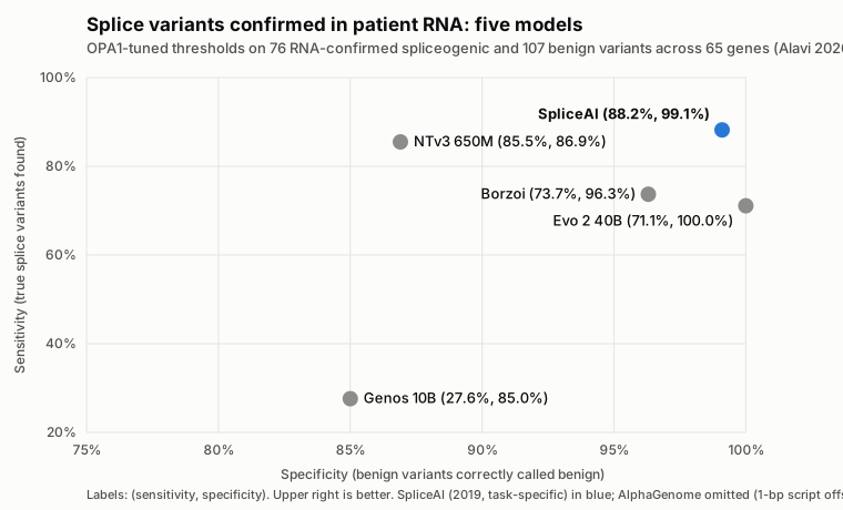
Figure 12. The Table 4 threshold-transfer results plotted as sensitivity against specificity across five models with valid variant coordinates. Upper right is better. Plotted by the author from Alavi's reported values.12
As Table 4 and Figure 12 show, transferring OPA1-tuned high-specificity thresholds across 65 genes exposes a trade-off between sensitivity and cross-gene generalisability: the 2019 task-specific tool SpliceAI59 retained both 88.2% sensitivity and 99.1% specificity, whereas Evo 2 40B13 kept 100% specificity at 71.1% sensitivity and post-trained NTv3 650M6 reached 85.5% sensitivity at 86.9% specificity (the initial October 2025 Genos 10B21 checkpoint scored 27.6% sensitivity, before BGI's December 2025 Genos-10B-v2 update22). Alavi also applied those same OPA1-tuned thresholds to 306 pathogenic OPA1 substitutions across every mutation class (missense, nonsense, splice-site, and untranslated region): pretrained-only DNA language models flagged most pathogenic variants regardless of mechanism (Evo 2 40B: 276/306, or 90.2%; pretrained NTv3 650M: 212/306, or 69.3%), acting as general sequence-constraint sensors, whereas post-training NTv3 650M on functional tracks narrowed positive calls to 77/306 (25.2%), in line with the ~25% splicing fraction and specialist models (SpliceAI: 75/306, or 24.5%; Borzoi:60 86/306, or 28.1%).1 Why is AlphaGenome omitted from Table 4 and Figure 12? Alavi's AlphaGenome scoring scripts subtracted 1 from each 1-based variant coordinate before calling AlphaGenome's 1-based Variant API, shifting every tested position one base to the left (issue #2),2 so the 56.6% sensitivity and 80.4% specificity reported in the preprint did not evaluate the intended variants. On valid coordinates, AlphaGenome's composite splicing score reached a ClinVar splice-region area under the precision-recall curve (auPRC) of 0.57 versus 0.55 for Pangolin61 in its own paper.16 Meanwhile, Illumina released SpliceAI2 on 8 October 2026:62 in its developers' preprint (11 October), SpliceAI2 beat SpliceAI, Pangolin, and AlphaGenome on a GTEx cryptic splice variant benchmark (auPRC of 0.77 vs. 0.66 for SpliceAI, 0.56 for Pangolin, and 0.54 for AlphaGenome's composite score or 0.63 with AlphaGenome's raw splice-site score) and on cryptic splice gains in blood RNA-seq from 5,435 Genomics England rare-disease participants (auPRC 0.59 vs. 0.48 for SpliceAI, 0.40 for Pangolin, and 0.36 for AlphaGenome, or 0.45 with AlphaGenome's raw splice-site score).62 My SpliceAI2 review and database extraction document those developer-reported figures; for clinical work today, prioritise splice candidates with SpliceAI59 or Pangolin61 and confirm in patient RNA with FRASER63 (Figure 13; splicing review).
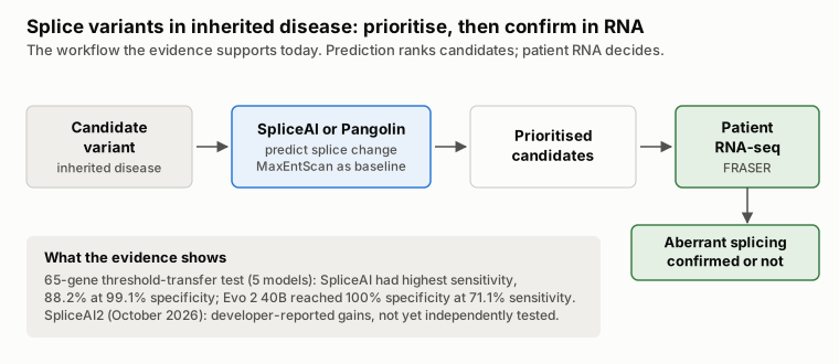
Figure 13. The splice-variant workflow supported by current evidence: predict to prioritise, then confirm in patient RNA.64596163 Figures from Table 4.1 Diagram by the author.
- Post-calling variant effect scoring (Oncology and Inherited): Once a variant is already called, scoring its functional impact is where foundation models look most competitive. In the EVEE preprint (version 4, July 2026), Pearce and colleagues trained a covariance-based probe on frozen Evo 2 7B embeddings and reached an AUROC of 0.991 on ClinVar indels versus 0.980 for CADD.65 For sequence-to-function models, the AlphaGenome Atlas preprint similarly collapses AlphaGenome's multi-track predictions into a precomputed AlphaGenome Variant Impact (AVI) score for every possible human SNV (under non-commercial research terms).17 Still, several EVEE authors co-authored Evo 2, its ClinVar embedding extraction took roughly 20,000 H100 GPU-hours,65 and Evo 2 does not win on every variant class: in its own paper it trails protein and alignment models (AlphaMissense,66 ESM-1b,67 and GPN-MSA68) on coding SNVs,13 and in the TraitGym regulatory benchmark, alignment-based models (CADD69 and GPN-MSA68) compare favourably across Mendelian and complex disease traits.70 In my companion evaluation on 3,893 experimentally measured BRCA1 single-nucleotide variants from Findlay and colleagues,71 zero-shot Evo 2 7B likelihood scoring beat the 2015 CADD v1.3 baseline bundled with the original dataset on noncoding variants (+0.077 AUROC), but that lead disappeared once compared against current CADD v1.769 (0.953 vs. 0.932; paired difference +0.021, 95% confidence interval -0.003 to +0.045) and SpliceAI59 (0.953 vs. 0.963; paired difference -0.011, 95% interval -0.025 to +0.003), while CADD v1.7 (0.892 vs. 0.840) and REVEL72 (0.867 vs. 0.785) clearly led on coding and missense variants (results and methods; full benchmark and cloud study).
Hardware, Memory, and Fine-Tuning Requirements Across DNA Models
The wider matched resource study across smaller DNA models remains incomplete (sizing protocol). In the meantime, Table 5 compiles what each model's authors report for inference and fine-tuning alongside my measured single-GPU figures for Evo 2 7B.
| Model | Reported or measured hardware and memory requirements |
|---|---|
| DNABERT-2 | Fine-tunes "on most consumer GPUs"3 |
| Nucleotide Transformer 2.5B | Weights take 9.5 GB; fine-tuning took 50 minutes on eight A100s (Methods)5 |
| NTv3 | Designed to run inference on 1 Mb windows on one A100 or H100; in mixed precision, the 8M model runs tens of kb on a laptop CPU6 |
| HyenaDNA 32k | Model card suggests a T4 (16 GB) to fine-tune and run73 |
| HyenaDNA 1M | Model card suggests an A100 80 GB to fine-tune and an A100 40 GB to run73 |
| Caduceus | Experiments ran on GPUs from an RTX 3090 to an A100 (Appendix F)10 |
| Evo 2 (7B, 20B, 40B) | 7B peaked at 16.8 GiB PyTorch allocated (20.8 GiB sampled device memory) at 8 kb on a 24 GB L4, 30.4 GiB at 33 kb on one 48 GB L40S or 80 GB H100, and ran out of memory at 131 kb on one 80 GB H100 (study repository; cloud study). The 1B, 20B, and 40B checkpoints require Hopper FP8 support;15 Arc reports 46 GB on one H100 for 20B (8 kb, 0.7 s/seq) and 95 GB across two H100s for 40B (1.5 s/seq)14 |
| AlphaGenome | Under 1 second per variant on an H100;16 the repository recommends at least an H10019 |
| GenomeOcean | Peak 21 GB (100M), 47 GB (500M) and 72 GB (4B) on an H100 when extracting embeddings in 16-bit (BF16) precision, with 5 kb inputs for the two smaller models and 50 kb for 4B; batch size not stated (Table 3)23 |
Table 5. GPU hardware, memory, and runtime figures across selected DNA sequence models.
Fine-tuning a compact or mid-sized model is far faster than pretraining: the Nucleotide Transformer team fine-tuned their 500M model in 20 minutes on average and their 2.5B model in 50 minutes on one node of eight A100s,5 and Hegde and colleagues independently fine-tuned NT 500M on roughly 89,000 expression quantitative trait locus (eQTL) variants in about 7.5 hours per five-epoch run on two NVIDIA TITAN Xp GPUs.74 When running large models such as Evo 2 7B for zero-shot likelihood scoring across cloud GPUs, note that low-precision bfloat16 and FP8 reductions are not associative across different GPU models: while two H100s on different clouds produced bit-identical BRCA1 scores, scoring the exact same container on an L40S shifted per-variant scores by a median of and flipped binary calls on 1.8% to 4.9% of variants across fixed thresholds, and a 24 GB L4 follow-up completed all 3,893 variants (AUROC 0.8772 vs. 0.8750 on H100) but missed the predefined Spearman 0.99 rank-agreement threshold at 0.9829—a cross-hardware drift eliminated by running in full 32-bit FP32 precision or locking the pipeline to a single validated GPU product (classification flips; L4 follow-up; full cloud operations and reproducibility study).
When to Use Zero-Shot, Frozen Embeddings, or Fine-Tuning
Saying "I used Evo 2" or "I used Nucleotide Transformer" does not specify how you generated a prediction. As Table 6 summarises, there are three distinct routes for turning a pretrained genomic foundation model into a predictor (Figure 14), and they differ sharply in labelled data requirements and compute cost.
| Route | What you calculate | What is trained on your labelled data |
|---|---|---|
| 1. Zero-shot likelihood scoring | The difference between the model's likelihood scores for the reference and alternate DNA sequences | No classifier is trained on your labels (though choosing a pass/fail cut-off still requires labelled validation data) |
| 2. Frozen embeddings plus a probe | Internal numerical vectors (embeddings) from the fixed model, fed into a simple classifier or regressor | Only the lightweight classifier ("probe") on top; the foundation model's weights stay fixed |
| 3. Fine-tuning | A task prediction after updating some or all of the foundation model's internal parameters | Both the task prediction head and selected parameters inside the foundation model |
Table 6. The three standard routes for turning a pretrained genomic foundation model into a task predictor, comparing what each route computes and what it trains on your labelled dataset.

Figure 14. What stays frozen and what is trained in each route from Table 6. Diagram by the author.
Start with Frozen Embeddings (Route 2) When:
You are building a custom sequence classifier and want a fast, inexpensive test of whether a foundation model adds signal over a classical baseline. Pass your sequences through the frozen model, apply mean pooling across the token vectors, and fit a simple classifier (such as logistic regression or a small multi-layer perceptron) on top. Remember that this probe is still a supervised predictor trained on your labels—it is not zero-shot prediction. In the Nucleotide Transformer paper, trained probes on frozen embeddings matched a task-specific supervised baseline (BPNet) on 5 of 18 tasks and beat it on 8 (Results; Supplementary Table 6).5 Always compare your probe against a simple non-foundation-model baseline on the exact same train/validation/test split.
Fine-Tune (Route 3) When:
A frozen-embedding probe leaves a clear accuracy gap and you have enough labelled examples to hold out a clean validation set separate from your final test set (Figure 15).
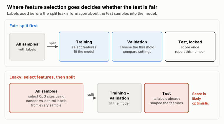
Figure 15. Feature selection, model fitting and threshold choice belong inside the training and validation data. The leaky pattern matches the limitation acknowledged in the CpGPT methylation study.40 Diagram by the author.
In the Nucleotide Transformer benchmark, fine-tuned models matched 6 of 18 supervised baselines and beat the remaining 12 (Fig. 2a,b; Supplementary Tables 7 and 9).5 Within the first-generation Nucleotide Transformer models, larger checkpoints pretrained on more diverse genomes fine-tuned better—though the second-generation 250M NT-v2 subsequently beat the 2.5B model at one-tenth the size.5
Parameter-Efficient Fine-Tuning: (IA)3 and LoRA
You rarely need to update all parameters in a foundation model. Parameter-efficient fine-tuning (PEFT) methods freeze the pretrained backbone and train only a tiny set of adapter weights (Figure 16):
- (IA)3 (used by Nucleotide Transformer) scales inner activations with learned vectors, adding trainable parameters equal to only about 0.1% of the model's parameters (Results and Methods, Fine-tuning).575
- LoRA76 (built into DNABERT-2's
finetune/train.pyscript viause_lora)77 injects low-rank update matrices into attention layers.
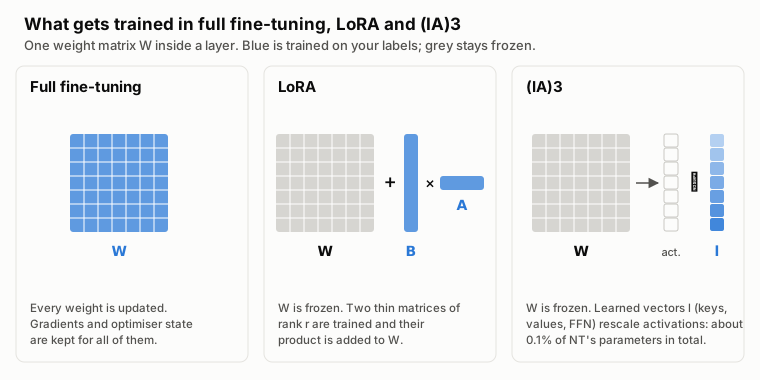
Figure 16. Which weights are trained in full fine-tuning, LoRA76 and (IA)3.755 Matrix sizes are schematic. Diagram by the author.
One hardware reality check: while updating 0.1% of the weights drastically shrinks optimizer-state and gradient memory, forward-pass activations still scale with sequence length and batch size—so always measure peak GPU memory on your longest sequences before committing to a training run.
Practical Decision Matrix
When selecting a candidate tool or model to test on your own validation split, match the choice to the clinical or research scenario:
- Calling somatic variants, RNA fusions, CNVs, or pathogens from raw reads:
- Prioritising splice variants in inherited disease:
- Use today: SpliceAI59 or Pangolin,61 followed by confirmation in patient RNA (FRASER63). When OPA1-tuned high-specificity thresholds were transferred across 65 genes in the only independent RNA-confirmed splice test, SpliceAI achieved the highest sensitivity (88.2% at 99.1% specificity) ahead of four newer genomic models (Table 4).1
- Scoring already-called coding or noncoding variants:
- Start with: Free precomputed scores from CADD v1.7,69 REVEL72 or AlphaMissense66 (for missense), GPN-MSA,68 and SpliceAI59 (or, for non-commercial research, precomputed AlphaGenome Variant Impact (AVI) scores from AlphaGenome Atlas17).
- To test a foundation model locally: The 24 GB L4 completed Evo 2 7B13 zero-shot likelihood scoring (Route 1) with 8 kb windows at about $0.76 per 1,000 variants including disk for the BRCA1 dataset (which shares reference windows), though its score-ranking agreement with the historical H100 reference missed the predefined threshold: verify numerical agreement as well as memory fit, or evaluate a supervised embedding probe (Route 2) on a held-out split (cloud setup and cost guide).
- Custom DNA sequence classification by window length (Figure 17):
- Short sequences (up to ~2–12 kb): DNABERT-2 (117M)3 or NT-v2 (50M–500M)5 using frozen embeddings, mean pooling,4 and a simple classifier probe (Route 2).
- Medium-to-long sequences (10 kb to 100 kb): Caduceus-Ph (up to 131 kb),104 NTv3,6 or a HyenaDNA checkpoint pretrained on 2 to 4 times your input length.7 Verify on validation data that wider context actually improves accuracy over a 2 kb window.
- Very long sequences (>100 kb) or sequence generation: NTv3 (designed for 1 Mb on one A100/H100)6 or Evo 213 (noting that Evo 2 7B needed more than one 80 GB GPU at 131 kb in standard single-GPU inference).
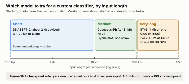
Figure 17. Starting models for a custom sequence classifier by input length, from the decision matrix above, with the HyenaDNA checkpoint rule.7 Diagram by the author.
What Scale Actually Buys You: Inside Evo and Evo 2
Why build 7-billion to 40-billion-parameter genomic models at all if smaller models handle short-sequence classification so well? The Evo and Evo 2 papers show what changes when you combine long-context architectures with genome-scale pretraining:
- Hybrid StripedHyena architecture: To avoid the scaling of pure dense attention while preserving the precision attention brings to local motifs, the original 7B Evo interleaves 29 Hyena convolutional layers with 3 rotary-attention layers (10%) (Figure 18, panel B).12
- From single genes to multi-gene systems: Pretrained on 300 billion nucleotide tokens from over 80,000 bacterial and archaeal genomes plus phage and plasmid sequences (1,000 times HyenaDNA's parameter count and 100 times its training data), Evo learned how genes co-occur across whole operons and mobile elements—allowing it to generate coding-rich sequences up to 650 kb long and outperform specialised RNA language models on zero-shot noncoding RNA fitness prediction.12
- Scaling across all domains of life in Evo 2: Because Evo saw only prokaryotic and phage DNA, its authors noted that its zero-shot predictions did not transfer well to human genes.12 Evo 2 scaled pretraining to more than 8.8 trillion nucleotides across bacteria, archaea, organelles, and eukaryotes (9.3 trillion tokens for the 40B model) with context windows up to 1 Mb.13 That cross-species, multi-domain training is what allows a single unsupervised model to score coding, noncoding, and splice-site mutations in BRCA1 without ever seeing a clinical variant label during training—even when task-specific supervised tools like REVEL, CADD v1.7, and SpliceAI still hold the edge on standard diagnostic benchmarks.
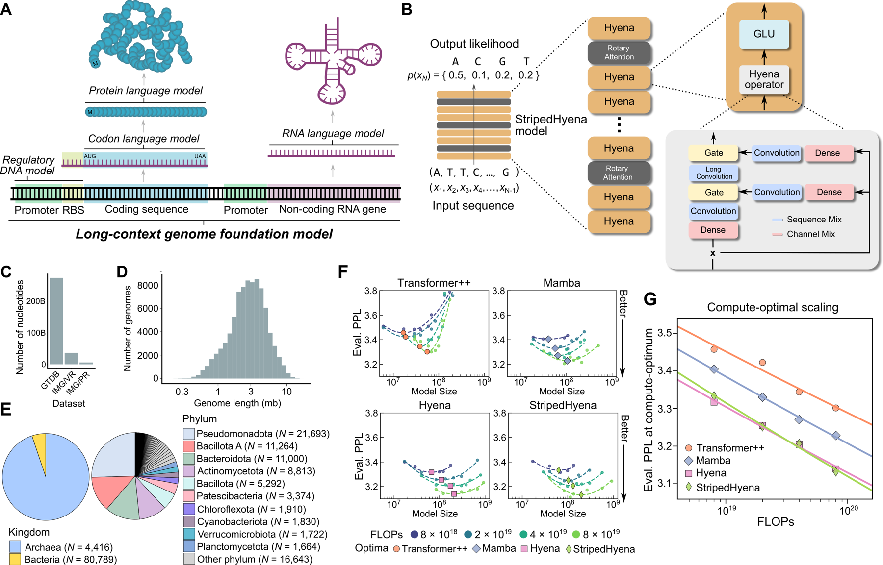
Figure 18. Evo's design and scaling study. (B) StripedHyena interleaves Hyena convolution layers with rotary attention layers. (F, G) In the authors' compute-matched comparison on DNA, StripedHyena and Hyena reached lower evaluation perplexity than Transformer++ and Mamba. Source: Nguyen E, et al., Sequence modeling and design from molecular to genome scale with Evo, bioRxiv (2024), Figure 1, CC BY 4.0; published in Science.12
What These Models Can't Do (Yet)
Before putting any genomic foundation model near a clinical pipeline, keep five boundaries in view:
- Benchmarks do not establish clinical validity. Neither published research benchmarks nor single-gene saturation-genome-editing studies validate an end-to-end clinical diagnostic test, and cross-GPU evaluations show that borderline variant classifications can flip when you change GPU models or floating-point precision (cloud reproducibility study).
- Context limits persist in practice. Even a 1-million-base window is only about 0.03% of a 3.2-billion-base human genome,7 and in standard single-GPU Evo 2 7B runs, a single 80 GB H100 ran out of memory at 131 kb (Figure 19). Chromosome-scale 3D regulation remains beyond single-GPU language model windows.
- Predictions are not explanations. Foundation models output log-likelihood shifts or high-dimensional embeddings, not auditable molecular mechanisms that a clinical scientist can sign out on a patient report.
- Pretraining genomes dictate what the model knows. The original Evo was trained strictly on prokaryotes and phages,12 limiting its human performance; always check which organisms and genomic elements a checkpoint saw during pretraining.
- Outdated baselines flatter new models. Always test against the current release of established tools on the same data split. On BRCA1, Evo 2's apparent noncoding win over 2015 CADD v1.3 vanished once compared against 2024 CADD v1.7 and SpliceAI.
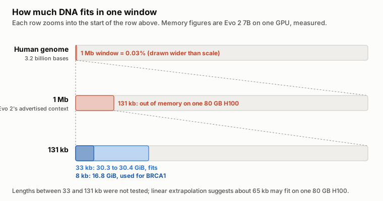
Figure 19. Evo 2 7B window sizes against the human genome, with the peak single-GPU memory measured in my companion cloud study. Diagram by the author.
Conclusion
If you are evaluating genomic foundation models for a diagnostic lab in 2026, anchor every decision to the clinical task, the prediction route, and a fair comparison against current baselines:
- Keep validated pipelines for calling and detection: For somatic variants, RNA fusions, CNVs, and pathogen identification, keep your established tools; across my eight workflow reviews, no foundation model has yet beaten them on clinical endpoints.
- Check free, current predictors before renting GPUs: On BRCA1, updating the comparator from CADD v1.3 to current CADD v1.7 and SpliceAI eliminated Evo 2 7B's apparent noncoding advantage, while REVEL and CADD v1.7 led on coding and missense variants.
- Start small, mean-pool, and test a frozen probe first: For custom DNA sequence classification, a 117M DNABERT-2 or 250M NT-v2 checkpoint with frozen mean-pooled embeddings (Route 2) is fast, cheap, and competitive with models 10 to 20 times larger.
- A 24 GB GPU can fit an 8 kb Evo 2 7B workload: The L4 completed all 3,893 BRCA1 variants at 8 kb with 20.8 GiB peak sampled device memory, but missed the predefined ranking-agreement threshold against the historical H100 reference. Similar AUROC does not establish interchangeable predictions.
- Treat the GPU and numerical precision as part of the method: When running a large model like Evo 2 7B (Route 1), budget for actual single-GPU memory limits (16.8 GiB allocated / 20.8 GiB sampled at 8 kb, about 30.4 GiB at 33 kb, OOM at 131 kb) and either pin the exact GPU model or use FP32 to prevent borderline variants from flipping calls across hardware (step-by-step Evo 2 cloud guide).
Self-supervised models that learn the statistical structure of raw DNA across trillions of nucleotides are a genuine scientific advance. Used thoughtfully—as candidate features and variant scorers tested rigorously against your lab's best existing baselines—they can sharpen how we prioritise variants and annotate regulatory sequence, without ever replacing experimental and clinical validation.
Sources
Numbered citations in the text refer to the primary references below: published papers, preprints, release notes, and model cards supporting specific claims. My companion evidence reviews and original experimental analyses are linked inline where used and listed together below. A machine-readable source manifest records every source alongside its type, version, and the exact claims it supports.
Companion evidence reviews. Each review records its literature search, primary study extractions, and limitations.
- Choosing a somatic variant caller
- Choosing an RNA fusion caller
- Confirming splice variants in patient RNA
- SpliceAI2
- Detecting cancer from cfDNA fragmentomics
- Detecting cancer from plasma DNA methylation
- Detecting and classifying copy-number variants
- DNA pathogen identification workflows
- RNA pathogen detection by sequencing
- Accelerating variant calling and genomic models
My analyses.
- Evo 2 7B on three cloud GPU offers: study repository and write-up
- BRCA1 comparison with current predictors: results and methods, reproduction script, and instructions and data terms
- Reproducibility across GPUs: classification flips and follow-up results
- Pretraining cost calculation: prices and inputs
- SpliceAI2 results: database extraction
- Completed L4 BRCA1 follow-up: measurements, scores and data terms and offline analysis bundle
- Wider matched resource study, incomplete: protocol
References
Footnotes
-
Alavi MV. Probing Genomic Foundation Models with Splice-Variant Perturbations. bioRxiv (2026). ↩ ↩2 ↩3 ↩4 ↩5 ↩6 ↩7
-
Alavi MV. Probing-genomic-foundation-models-2026 issue #2: 1-base coordinate offset in
2c8_alphagenome_splicescorer.pyand2c8_alphagenome_junctionscorer.py. GitHub (2026). ↩ ↩2 ↩3 ↩4 -
Zhou Z, et al. DNABERT-2: Efficient Foundation Model and Benchmark For Multi-Species Genome. ICLR 2024. ↩ ↩2 ↩3 ↩4 ↩5 ↩6 ↩7
-
Feng H, et al. Benchmarking DNA foundation models for genomic and genetic tasks. Nature Communications 16, 10780 (2025). ↩ ↩2 ↩3 ↩4 ↩5 ↩6 ↩7 ↩8 ↩9
-
Dalla-Torre H, et al. Nucleotide Transformer: building and evaluating robust foundation models for human genomics. Nature Methods 22, 287 to 297 (2025). ↩ ↩2 ↩3 ↩4 ↩5 ↩6 ↩7 ↩8 ↩9 ↩10 ↩11 ↩12
-
Boshar S, et al. A foundational model for joint sequence-function multi-species modeling at scale for long-range genomic prediction. bioRxiv (2025). Introduces NTv3. ↩ ↩2 ↩3 ↩4 ↩5 ↩6 ↩7
-
Nguyen E, et al. HyenaDNA: Long-Range Genomic Sequence Modeling at Single Nucleotide Resolution. NeurIPS 2023. ↩ ↩2 ↩3 ↩4 ↩5 ↩6 ↩7 ↩8 ↩9 ↩10
-
Liu Z, et al. GenBench: A Benchmarking Suite for Systematic Evaluation of Genomic Foundation Models. arXiv (2024). ↩ ↩2 ↩3 ↩4 ↩5 ↩6 ↩7 ↩8
-
Dick JM. BreCol: Benchmarking Classical and Deep-Learning Methods for Microbiome-Based Cancer Detection. arXiv (2026). ↩
-
Schiff Y, et al. Caduceus: Bi-Directional Equivariant Long-Range DNA Sequence Modeling. ICML 2024. ↩ ↩2 ↩3 ↩4 ↩5
-
Kuleshov group. Caduceus checkpoints on Hugging Face; the 131k checkpoints have 7,725,312 parameters in their model metadata, for example caduceus-ph_seqlen-131k_d_model-256_n_layer-16. ↩
-
Nguyen E, et al. Sequence modeling and design from molecular to genome scale with Evo. Science 386, eado9336 (2024). ↩ ↩2 ↩3 ↩4 ↩5 ↩6
-
Brixi G, et al. Genome modelling and design across all domains of life with Evo 2. Nature 652, 1349 to 1361 (2026). ↩ ↩2 ↩3 ↩4 ↩5 ↩6 ↩7 ↩8
-
Arc Institute. Evo 2 release v0.5.0: 20B model and hardware notes. GitHub (2026). ↩ ↩2
-
Arc Institute. Evo 2 README: requirements. GitHub. ↩ ↩2
-
Avsec Ž, et al. Advancing regulatory variant effect prediction with AlphaGenome. Nature 649, 1206 to 1218 (2026). ↩ ↩2 ↩3 ↩4
-
Cheng J, Taylor J, Nicolaisen L, et al. AlphaGenome Atlas: in silico mutagenesis of the entire human genome. medRxiv (2026). Introduces the AlphaGenome Variant Impact (AVI) score. ↩ ↩2 ↩3
-
Google DeepMind. AlphaGenome API README and terms of use. GitHub. ↩
-
Google DeepMind. AlphaGenome model weights README. GitHub. ↩ ↩2
-
Fishman V, et al. GENA-LM: a family of open-source foundational DNA language models for long sequences. Nucleic Acids Research 53, gkae1310 (2025). ↩
-
Lin A, et al. Genos: a human-centric genomic foundation model. GigaScience 14, giaf132 (2025). ↩ ↩2 ↩3
-
BGI-HangzhouAI. Genos-10B-v2 model card. Hugging Face (released 18 December 2025). ↩ ↩2
-
Yu M, et al. FP8 Inference in Genomic Foundation Models: Theoretical vs. Realized Speedups on GenomeOcean. bioRxiv (2026). ↩ ↩2
-
Runpod GPU catalogue, secure-cloud on-demand prices, read through the Runpod API on 13 October 2026. My recorded prices and calculation; prices change, and the live list is on Runpod's pricing page. ↩
-
Benjamin D, et al. Calling somatic SNVs and indels with Mutect2. bioRxiv (2019). ↩ ↩2
-
Park J, et al. Accurate somatic small variant discovery for multiple sequencing technologies with DeepSomatic. Nature Biotechnology (2025). ↩
-
Kim S, et al. Strelka2: fast and accurate calling of germline and somatic variants. Nature Methods 15, 591 to 594 (2018). ↩
-
Hasan M. Prospectively frozen external benchmarking reveals benchmark-context dependence in somatic variant calling. Research Square preprint (2026). ↩
-
Wang M, et al. SomaticCombiner: improving the performance of somatic variant calling based on evaluation tests and a consensus approach. Scientific Reports 10, 12898 (2020). ↩
-
Behera S, et al. Comprehensive genome analysis and variant detection at scale using DRAGEN. Nature Biotechnology 43, 1177 to 1191 (2025). ↩
-
Illumina. DRAGEN v4.4 somatic mode documentation. ↩
-
Haas BJ, et al. Accuracy assessment of fusion transcript detection via read-mapping and de novo fusion transcript assembly-based methods. Genome Biology 20, 213 (2019). Introduces STAR-Fusion. ↩ ↩2
-
Uhrig S, et al. Accurate and efficient detection of gene fusions from RNA sequencing data. Genome Research 31, 448 to 460 (2021). Introduces Arriba. ↩ ↩2
-
Tamura Z, et al. Comparison of gene fusion detection algorithms reveals frequently overlooked driver fusions in hematologic malignancies. npj Precision Oncology 10, 81 (2026). ↩
-
Cristiano S, et al. Genome-wide cell-free DNA fragmentation in patients with cancer. Nature 570, 385 to 389 (2019). Introduces DELFI. ↩
-
Xu Y, et al. Toward generalizable prediction of cancer signal using a cell-free DNA language model. Cell Reports Medicine 7, 102866 (2026). Introduces Fragmentia-AI. ↩
-
Adalsteinsson VA, et al. Scalable whole-exome sequencing of cell-free DNA reveals high concordance with metastatic tumors. Nature Communications 8, 1324 (2017). Introduces ichorCNA. ↩
-
Moss J, et al. Comprehensive human cell-type methylation atlas reveals origins of circulating cell-free DNA in health and disease. Nature Communications 9, 5068 (2018). Introduces MethAtlas. ↩
-
de Lima Camillo LP, et al. CpGPT: a foundation model for DNA methylation. bioRxiv (2024). ↩
-
Xu Y, Feng Q. An Evaluation of DMR-Informed Fine-Tuning of Tissue Array-Pretrained CpGPT for Gastrointestinal Cancer Classification Using cfDNA Targeted Methylation. medRxiv (2026). Version 1, 29 July 2026. ↩ ↩2 ↩3
-
Plagnol V, et al. A robust model for read count data in exome sequencing experiments and implications for copy number variant calling. Bioinformatics 28, 2747 to 2754 (2012). Introduces ExomeDepth. ↩ ↩2
-
Abyzov A, et al. CNVnator: an approach to discover, genotype, and characterize typical and atypical CNVs from family and population genome sequencing. Genome Research 21, 974 to 984 (2011). ↩ ↩2
-
Geoffroy V, et al. AnnotSV: an integrated tool for structural variations annotation. Bioinformatics 34, 3572 to 3574 (2018). ↩
-
Gurbich TA, Ilinsky VV. ClassifyCNV: a tool for clinical annotation of copy-number variants. Scientific Reports 10, 20375 (2020). ↩
-
Hwang J, et al. Improving CNV Detection Performance Except for Software-Specific Problematic Regions. Genes 17, 105 (2026). ↩
-
Zhang Y, Zhang X, Chen D. Can automated copy number variation pathogenicity prediction tools replace manual review under the ACMG framework? A clinical validation. Global Medical Genetics 100096 (2026). ↩
-
Wood DE, Lu J, Langmead B. Improved metagenomic analysis with Kraken 2. Genome Biology 20, 257 (2019). ↩ ↩2
-
Li H. Minimap2: pairwise alignment for nucleotide sequences. Bioinformatics 34, 3094 to 3100 (2018). ↩ ↩2
-
Huson DH, et al. MEGAN-LR: new algorithms allow accurate binning and easy interactive exploration of metagenomic long reads and contigs. Biology Direct 13, 6 (2018). ↩ ↩2
-
Portik DM, Brown CT, Pierce-Ward NT. Evaluation of taxonomic classification and profiling methods for long-read shotgun metagenomic sequencing datasets. BMC Bioinformatics 23, 541 (2022). ↩
-
Mock F, et al. Taxonomic classification of DNA sequences beyond sequence similarity using deep neural networks. PNAS 119, e2122636119 (2022). Introduces BERTax. ↩
-
Peres da Silva R, et al. MetageNN: a memory-efficient neural network taxonomic classifier robust to sequencing errors and missing genomes. BMC Bioinformatics 25, 153 (2024). ↩ ↩2
-
Kim D, et al. Centrifuge: rapid and sensitive classification of metagenomic sequences. Genome Research 26, 1721 to 1729 (2016). ↩
-
Tan JK, et al. Laboratory validation of a clinical metagenomic next-generation sequencing assay for respiratory virus detection and discovery. Nature Communications 15, 9016 (2024). Evaluates SURPI+ on respiratory RNA specimens. ↩ ↩2
-
Kalantar KL, et al. IDseq—An open source cloud-based pipeline and analysis service for metagenomic pathogen detection and monitoring. GigaScience 9, giaa111 (2020). Introduces IDseq (now CZ ID). ↩ ↩2
-
Marangoni S, et al. GeNePi: a graphics processing unit enhanced next-generation bioinformatics pipeline for whole-genome sequencing analysis. Briefings in Bioinformatics 27, bbag001 (2026). ↩
-
O'Connell K, et al. Accelerating genomic workflows using NVIDIA Parabricks. BMC Bioinformatics 24, 221 (2023). ↩
-
Samarakoon P, et al. Benchmarking accelerated next-generation sequencing analysis pipelines. Bioinformatics Advances 5, vbaf085 (2025). ↩ ↩2
-
Jaganathan K, et al. Predicting Splicing from Primary Sequence with Deep Learning. Cell 176, 535 to 548 (2019). ↩ ↩2 ↩3 ↩4 ↩5 ↩6 ↩7
-
Linder J, et al. Predicting RNA-seq coverage from DNA sequence as a unifying model of gene regulation. Nature Genetics 57, 949 to 961 (2025). Introduces Borzoi. ↩ ↩2
-
Zeng T, Li YI. Predicting RNA splicing from DNA sequence using Pangolin. Genome Biology 23, 103 (2022). ↩ ↩2 ↩3 ↩4
-
Jaganathan K, et al. A unified framework for quantitative splicing and transcript prediction. bioRxiv (2026). Introduces SpliceAI2. Release date from Illumina's press release, 8 October 2026. ↩ ↩2
-
Mertes C, et al. Detection of aberrant splicing events in RNA-seq data using FRASER. Nature Communications 12, 529 (2021). ↩ ↩2 ↩3
-
Yeo G, Burge CB. Maximum entropy modeling of short sequence motifs with applications to RNA splicing signals. Journal of Computational Biology 11, 377 to 394 (2004). Introduces MaxEntScan. ↩
-
Pearce MT, et al. Interpretable variant effect prediction from genomic foundation model representations. bioRxiv (2026). Introduces EVEE. Version 4, 11 July 2026. ↩ ↩2
-
Cheng J, et al. Accurate proteome-wide missense variant effect prediction with AlphaMissense. Science 381, eadg7492 (2023). ↩ ↩2
-
Brandes N, et al. Genome-wide prediction of disease variant effects with a deep protein language model. Nature Genetics 55, 1512 to 1522 (2023). Evaluates ESM-1b on human coding variants. ↩
-
Benegas G, et al. A DNA language model based on multispecies alignment predicts the effects of genome-wide variants. Nature Biotechnology 43, 1960 to 1965 (2025). Introduces GPN-MSA. ↩ ↩2 ↩3
-
Schubach M, et al. CADD v1.7: using protein language models, regulatory CNNs and other nucleotide-level scores to improve genome-wide variant predictions. Nucleic Acids Research 52, D1143 to D1154 (2024). ↩ ↩2 ↩3
-
Benegas G, et al. Benchmarking DNA Sequence Models for Causal Regulatory Variant Prediction in Human Genetics. bioRxiv (2025). Introduces TraitGym. ↩
-
Findlay GM, et al. Accurate classification of BRCA1 variants with saturation genome editing. Nature 562, 217 to 222 (2018). ↩
-
Ioannidis NM, et al. REVEL: An Ensemble Method for Predicting the Pathogenicity of Rare Missense Variants. American Journal of Human Genetics 99, 877 to 885 (2016). The study used REVEL v1.3 scores. ↩ ↩2
-
LongSafari. HyenaDNA model card. Hugging Face. ↩ ↩2
-
Hegde M, et al. Reaping the Fruits of LLM Pruning: Towards Small Language Models for Efficient Non-Coding Variant Effect Prediction. Genes 16, 1358 (2025). ↩
-
Liu H, et al. Few-Shot Parameter-Efficient Fine-Tuning is Better and Cheaper than In-Context Learning. NeurIPS 2022. Introduces (IA)3. ↩ ↩2
-
Hu EJ, et al. LoRA: Low-Rank Adaptation of Large Language Models. ICLR 2022. ↩ ↩2
-
MAGICS Lab. DNABERT-2 fine-tuning script,
finetune/train.py. GitHub, commit b3337f3 (21 August 2024). ↩
Help improve this article
Found an error or a better source? Leave a note here, or highlight a passage to comment on it.